gene.odm, grna.odm, and sceptre_object.rds files — are contained in the shared storage space.
In this chapter we delve deeper into the sceptre Nextflow pipeline. First, we review clusters and explain how information flows through the sceptre Nextflow pipeline on a cluster. Next, we describe the structure of a typical sceptre Nextflow submission script. Then, we provide a few examples of common analysis workflows in the context of the Nextflow pipeline. Finally, we describe how to run a massive-scale trans analysis using the Nextflow pipeline.
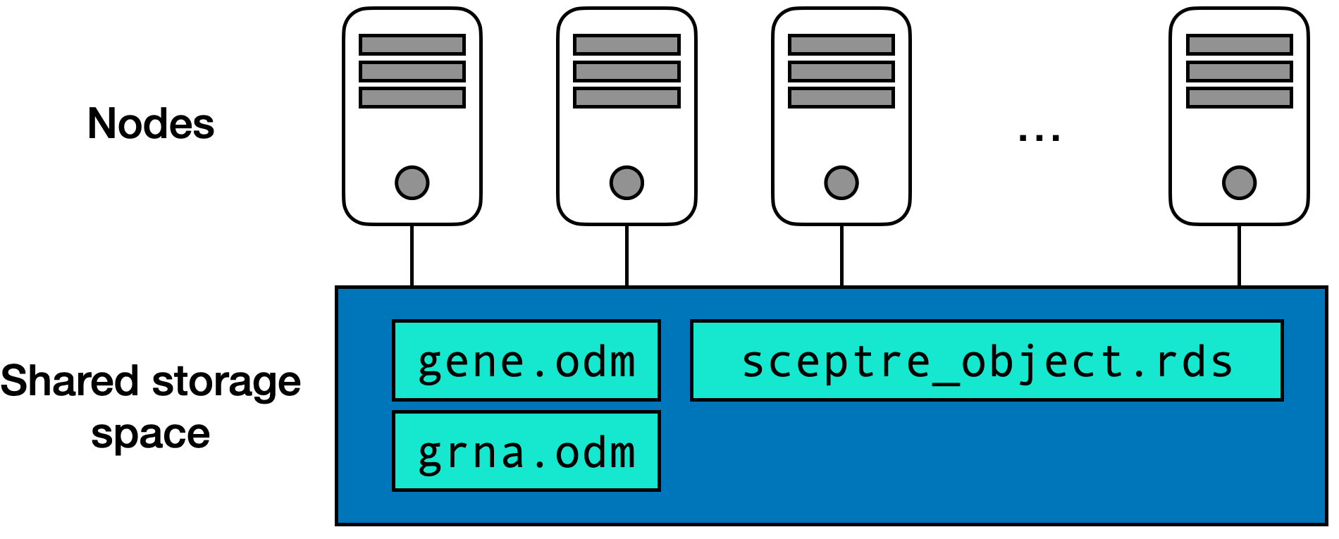
A computing cluster is of a collection of computers, also known as nodes, that work in concert to carry out a large computation. Figure 8.1 illustrates the structure of a typical computing cluster. The cluster contains dozens or even hundreds of nodes, with each node harboring multiple processors. Processors are the core units that execute code. Furthermore, all nodes are linked to a common storage area where files are kept. For instance, specific data files like gene.odm, grna.odm, and sceptre_object.rds are stored in this shared space.
The process of performing a computation on a cluster involves several steps. Initially, each processor loads only the part of the data that it needs for its portion of the overall computation. Then, each processor processes this part of the data and saves the results back to the shared storage area. Once all processors complete their tasks, another processor retrieves these results from the shared space and merges them into a final result. Typically, the processors are spread across different nodes and thus do not directly interact with each other; rather, they coordinate through the shared storage space. This method of distributing tasks among independent processors and later combining their outputs is known as a scatter-gather operation. The sceptre Nextflow pipeline consists of multiple scatter-gather chained together.
gene.odm, grna.odm, and sceptre_object.rds files — are contained in the shared storage space.
A graph illustrating the flow of information through the sceptre Nextflow pipeline is depicted in Figure 8.2. The steps of the pipeline as outlined in Figure 7.1 (i.e., “set analysis parameters,” “assign gRNAs,” “run quality control,” “run calibration check,” “run power check,” and “run discovery analysis”) are all present in the graph. The computation is parallelized at four points: “assign gRNAs,” “run calibration check,” “run power check,” and “run discovery analysis.” The “assign gRNAs” step is parallelized according to the following scatter-gather strategy. First, the gRNAs are partitioned into p distinct “pods.” For example, if the data contain 100 gRNAs, and if p = 5 pods are in use, then each pod is assigned 20 distinct gRNAs. Next, each pod is mapped to one of p processors, and each processor performs the gRNA-to-cell assignments for the gRNAs within the pod to which it has been assigned. Finally, the gRNA-to-cell assignments are combined across pods, yielding a single binary gRNA-to-cell assignment matrix. The user selects the number of gRNAs to assign to each pod, which in turn determines the number of pods p.
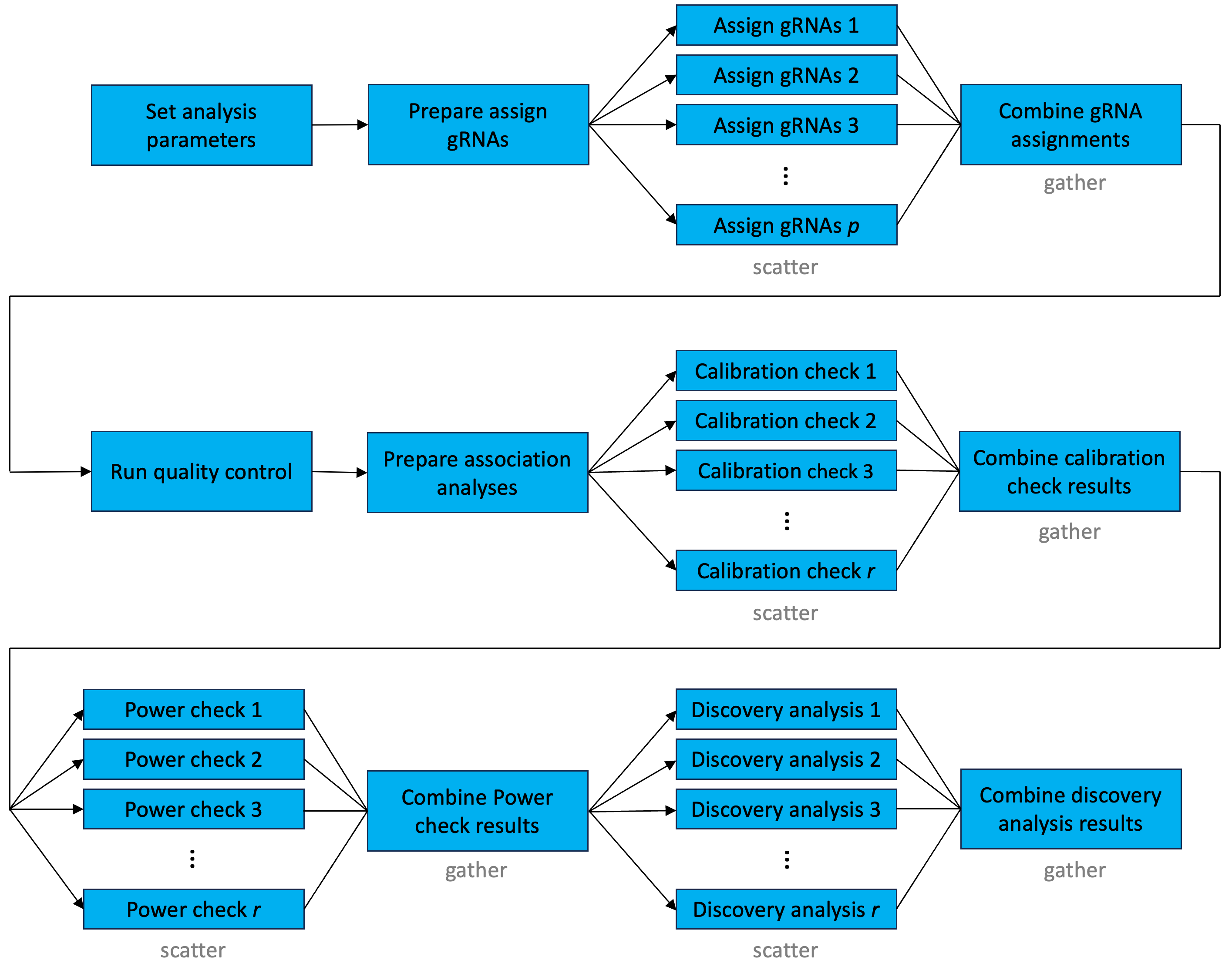
sceptre Nextflow pipeline. The pipeline consists of several scatter-gather operations chained together, with parallelization at the gRNA assignment and association testing steps.
The “run calibration check,” “run power check,” and “run discovery analysis” steps are parallelized using a similar strategy. First, the target-response pairs are partitioned into r distinct pods. Next, the pods are mapped to r processors, and each processor carries out the target-to-response association tests for the pairs in the pod to which it has been assigned. Finally, the results are combined across pods, and a multiplicity correction (e.g., the BH procedure) is applied to the entire set of p-values. Again, the user selects the number of pairs to assign to each pod, which in turn determines r. In summary the gRNA-to-cell assignments are parallelized at the level of the gRNA, and the target-to-response association tests are parallelized at the level of the target-response pair. (If the “maximum” gRNA assignment strategy is used, then the gRNA-to-cell assignment step is not parallelized. Rather, the gRNA-to-cell assignments are carried out “behind the scenes” as part of the data import step.)
An example sceptre Nextflow pipeline launch script is as follows.
launch_script.sh
#$ -l m_mem_free=4G
#$ -pe openmp 2
export NXF_OPTS="-Xms500M -Xmx4G"

##########################
# REQUIRED INPUT ARGUMENTS
##########################
data_directory=$HOME"/sceptre_data/"
# sceptre object
sceptre_object_fp=$data_directory"sceptre_object.rds"
# response ODM
response_odm_fp=$data_directory"gene.odm"
# grna ODM
grna_odm_fp=$data_directory"grna.odm"

###################
# OUTPUT DIRECTORY:
##################
output_directory=$HOME"/sceptre_outputs"

#################
# Invoke pipeline
#################
nextflow run timothy-barry/sceptre-pipeline -r main \
 --sceptre_object_fp $sceptre_object_fp \
 --response_odm_fp $response_odm_fp \
 --grna_odm_fp $grna_odm_fp \
 --output_directory $output_directory \
 --grna_assignment_method mixture \
 --response_n_umis_range_lower 0.05 \
 --response_n_umis_range_uppper 0.95 \
 --grna_integration_strategy singleton \
 --pair_pod_size 1000 \
 --grna_pod_size 25 \
 --combine_assign_grnas_memory 8GB \
 --combine_assign_grnas_time 5m
We describe each component of this script line-by-line. The first few lines relate to resource requests for the driver process. We request four gigabytes of memory (#$ -l m_mem_free=4G) and two CPUs (#$ -pe openmp 2) for the driver. Additionally, we specify that the “Java virtual machine” — the application responsible for executing the driver — is to use no fewer than 500 megabytes of memory and no more than to four gigabytes of memory via the line export NXF_OPTS="-Xms500M -Xmx4G". (This line is optional, but it helps prevent the Nextflow driver from using too much memory.) Finally, the scheduler may require us to submit a wall time request, in which case we should include a wall time request at the top of launch_script.sh; the relevant command on SGE is #$ -l h_rt. If we were on a SLURM cluster instead of an SGE cluster, the first few lines of launch_script.sh would look roughly as follows:
#SBATCH --ntasks=1
#SBATCH --cpus-per-task=2
#SBATCH --mem=4G
#SBATCH --time=05:00:00
export NXF_OPTS="-Xms500M -Xmx4G"
Next, we set the variables sceptre_object_fp, response_odm_fp, and grna_odm_fp to the file paths of the sceptre_object.rds file, the gene.odm file, and the grna.odm file, respectively. We also set output_directory to the file path of the directory in which to write the results. These variables are defined in terms of $HOME as opposed to the shorthand ~, as $HOME contains the absolute file path to the home directory, and Nextflow is more adept at handling absolute file paths than relative file paths.
Finally, we invoke the Nextflow pipeline via the command nextflow run timothy-barry/sceptre-pipeline -r main. (timothy-barry/sceptre-pipeline is the current location of the sceptre Nextflow pipeline on Github; we plan to move the pipeline into the nf-core repository in the future.) We specify arguments to the pipeline via the syntax --argument value, where argument is the name of an argument and value is the value to assign to the argument. In the above script we organize the arguments such that each argument is on its own line, but this is not necessary. The sceptre pipeline has four required arguments: sceptre_object_fp, response_odm_fp, grna_odm_fp, and output_directory (described above). The pipeline additionally supports a variety of optional arguments. About half of the optional arguments are “statistical” in that they govern how the statistical methods are to be deployed to analyze the data. For example, above, we indicate that the pipeline is to use the “mixture” method to assign gRNAs to cells via --grna_assignment_method. Additionally, we alter the default cellwise QC thresholds via --response_n_umis_range_lower 0.05 and --response_n_umis_range_uppper 0.95. Finally, we indicate that the pipeline is to use the “singleton” gRNA integration strategy via --grna_integration_strategy singleton.
The other half of the optional arguments are “computational” in that they control how the computation is organized and executed. For example, we set the gRNA pod size to 25 and the target-response pair pod size to 1,000 via –pair_pod_size 1000 and –-grna_pod_size 25, respectively. Each process in the pipeline submits a time and memory allocation request to the scheduler. These resource requests are set to reasonable defaults, but we manually can override the defaults for a given process (or processes) on the command line. For example, we request eight gigabytes of memory and five minutes of wall time for the “Combine assign gRNAs” process via –-combine_assign_grnas_memory 8GB and –-combine_assign_grnas_time 5m, respectively.
All of the sceptre Nextflow pipeline arguments are enumerated and described in Section 9.2 of the addendum to Part II of this book. We recommend that users skim through this section and reference it as needed.
We describe a few common workflows in the context of the sceptre Nextflow pipeline.
A common workflow is to advance through the pipeline one step at a time (Section 7.9), adjusting the input arguments as necessary on the basis of the intermediate outputs. For example, suppose that we decide to implement an aggressive cellwise QC strategy, setting --response_n_umis_range_lower and --response_n_umis_range_uppper to0.2 and 0.8, respectively, so as to clip the tails of the response_n_umis distribution at the 20th percentile and 80 percentile. Additionally, we set --pipeline_stop to run_qc to stop the pipeline at the “Run QC” step.
#!/bin/bash
# Limit NF driver to 4 GB memory
export NXF_OPTS="-Xms500M -Xmx4G"

##########################
# REQUIRED INPUT ARGUMENTS
##########################
data_directory=$HOME"/sceptre_data/"
# sceptre object
sceptre_object_fp=$data_directory"sceptre_object.rds"
# response ODM
response_odm_fp=$data_directory"gene.odm"
# grna ODM
grna_odm_fp=$data_directory"grna.odm"

###################
# OUTPUT DIRECTORY:
##################
output_directory=$HOME"/sceptre_outputs"

#################
# Invoke pipeline
#################
nextflow run timothy-barry/sceptre-pipeline -r main \
 --sceptre_object_fp $sceptre_object_fp \
 --response_odm_fp $response_odm_fp \
 --grna_odm_fp $grna_odm_fp \
 --output_directory $output_directory \
 --pair_pod_size 1000 \
 --grna_pod_size 25 \
 --response_n_umis_range_lower 0.2 \
 --response_n_umis_range_uppper 0.8 \
 --pipeline_stop run_qc
We launch the pipeline.
terminal
qsub launch.sh # or sbatch or bash, etc.An inspection of the “Response N UMIs” panel of plot_covariates.png suggests that we have clipped the tails a too extreme a location.
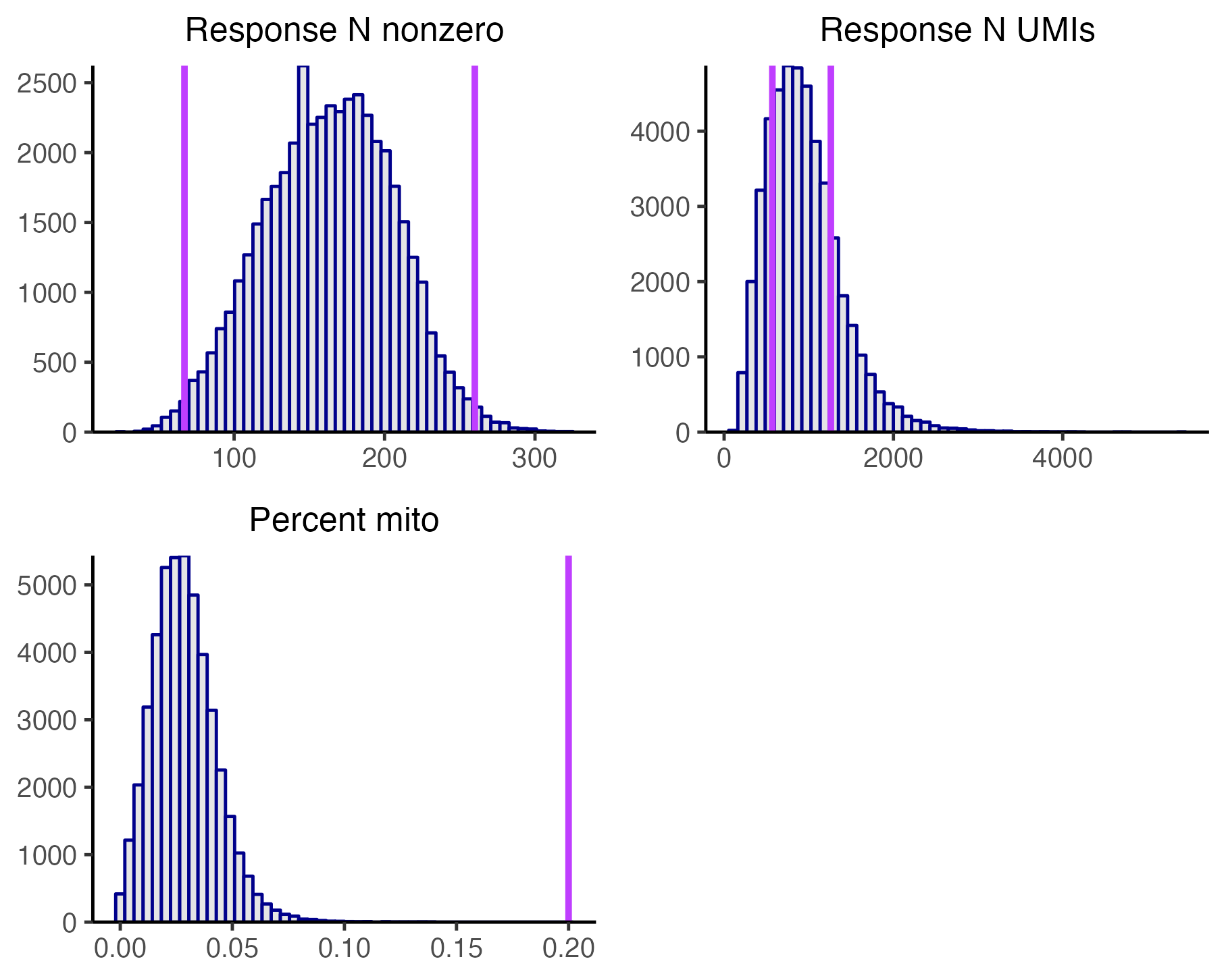
Thus, we relax the cellwise QC thresholds slightly, setting --response_n_umis_range_lower and --response_n_umis_range_uppper to0.1 and 0.9, respectively. Additionally, we pass the -resume flag to the pipeline to avoid recomputing the gRNA-to-cell assignments.
#!/bin/bash
# Limit NF driver to 4 GB memory
export NXF_OPTS="-Xms500M -Xmx4G"

##########################
# REQUIRED INPUT ARGUMENTS
##########################
data_directory=$HOME"/sceptre_data/"
# sceptre object
sceptre_object_fp=$data_directory"sceptre_object.rds"
# response ODM
response_odm_fp=$data_directory"gene.odm"
# grna ODM
grna_odm_fp=$data_directory"grna.odm"

###################
# OUTPUT DIRECTORY:
##################
output_directory=$HOME"/sceptre_outputs"

#################
# Invoke pipeline
#################
nextflow run timothy-barry/sceptre-pipeline -r main \
 --sceptre_object_fp $sceptre_object_fp \
 --response_odm_fp $response_odm_fp \
 --grna_odm_fp $grna_odm_fp \
 --output_directory $output_directory \
 --pair_pod_size 1000 \
 --grna_pod_size 25 \
 --response_n_umis_range_lower 0.1 \
 --response_n_umis_range_uppper 0.9 \
 --pipeline_stop run_qc \
 -resume
This approach — i.e., passing a set of candidate arguments to the pipeline, examining the output of the pipeline, and then updating the candidate arguments as necessary — is applicable to all steps of the pipeline.
The Nextflow pipeline may fail. This most commonly occurs when a process has exceeded its time and/or memory allocation. We provide an example of a pipeline failure and show how to resolve the failure. Consider the following submission script, in which we request only one MB of memory for the “Run association analysis” processes.
#!/bin/bash
# Limit NF driver to 4 GB memory
export NXF_OPTS="-Xms500M -Xmx4G"

##########################
# REQUIRED INPUT ARGUMENTS
##########################
data_directory=$HOME"/sceptre_data/"
# sceptre object
sceptre_object_fp=$data_directory"sceptre_object.rds"
# response ODM
response_odm_fp=$data_directory"gene.odm"
# grna ODM
grna_odm_fp=$data_directory"grna.odm"

###################
# OUTPUT DIRECTORY:
##################
output_directory=$HOME"/sceptre_outputs"

#################
# Invoke pipeline
#################
nextflow run timothy-barry/sceptre-pipeline -r main -resume \
 --sceptre_object_fp $sceptre_object_fp \
 --response_odm_fp $response_odm_fp \
 --grna_odm_fp $grna_odm_fp \
 --output_directory $output_directory \
 --pair_pod_size 1000 \
 --grna_pod_size 25 \
 --run_association_analysis_memory 1MB
We submit this script to the scheduler.
terminal, cluster
qsub launch.sh # or sbatch, etcThe job fails with the following log file.
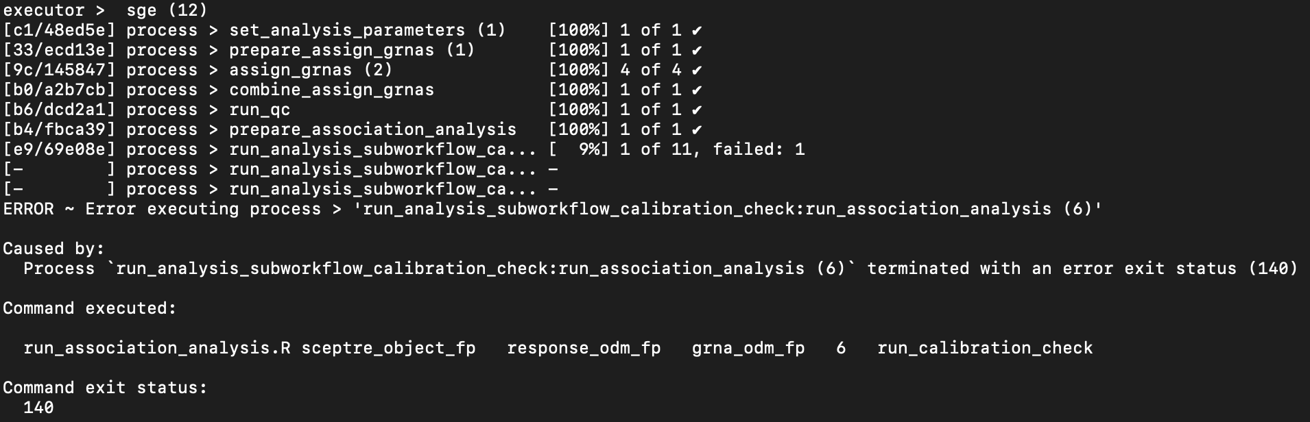
We see that there was an error executing the process run_analysis_subworkflow_calibration_check:run_association_analysis, which is the calibration check process. Moreover, the process failed with exit code of 140, which, on an SGE cluster, indicates that the process exceeded its memory allocation. To resolve this issue, we increase the memory request of the “Run association analysis” processes to 4GB, as follows.
#!/bin/bash
# Limit NF driver to 4 GB memory
export NXF_OPTS="-Xms500M -Xmx4G"

##########################
# REQUIRED INPUT ARGUMENTS
##########################
data_directory=$HOME"/sceptre_data/"
# sceptre object
sceptre_object_fp=$data_directory"sceptre_object.rds"
# response ODM
response_odm_fp=$data_directory"gene.odm"
# grna ODM
grna_odm_fp=$data_directory"grna.odm"

###################
# OUTPUT DIRECTORY:
##################
output_directory=$HOME"/sceptre_outputs"

#################
# Invoke pipeline
#################
nextflow run timothy-barry/sceptre-pipeline -r main -resume \
 --sceptre_object_fp $sceptre_object_fp \
 --response_odm_fp $response_odm_fp \
 --grna_odm_fp $grna_odm_fp \
 --output_directory $output_directory \
 --pair_pod_size 1000 \
 --grna_pod_size 25 \
 --run_association_analysis_memory 4GB
Now, the pipeline runs without issue. Determining the exact cause of a pipeline failure may take some sleuthing. In addition to examining the log file associated with the driver process, investigating the specific job that failed — through, e.g., a call to qacct on SGE or sacct on SLURM — can provide helpful information.
One can skip the calibration check and proceed straight to the power check and discovery analysis by setting --n_calibration_pairs to 0, as follows.
#!/bin/bash
# Limit NF driver to 4 GB memory
export NXF_OPTS="-Xms500M -Xmx4G"

##########################
# REQUIRED INPUT ARGUMENTS
##########################
data_directory=$HOME"/sceptre_data/"
# sceptre object
sceptre_object_fp=$data_directory"sceptre_object.rds"
# response ODM
response_odm_fp=$data_directory"gene.odm"
# grna ODM
grna_odm_fp=$data_directory"grna.odm"

###################
# OUTPUT DIRECTORY:
##################
output_directory=$HOME"/sceptre_outputs"

#################
# Invoke pipeline
#################
nextflow run timothy-barry/sceptre-pipeline -r main -resume \
 --sceptre_object_fp $sceptre_object_fp \
 --response_odm_fp $response_odm_fp \
 --grna_odm_fp $grna_odm_fp \
 --output_directory $output_directory \
 --pair_pod_size 1000 \
 --grna_pod_size 25 \
--n_calibration_pairs 0The sceptre Nextflow pipeline provides a special option for carrying out a massive-scale trans analysis in which each target is tested for association against each response. We call this special option the trans interface to the pipeline. The trans interface is an appropriate strategy for conducting a trans analysis when the number of trans pairs (i.e., the number of targets times the number of responses) exceeds 10 million, which is the maximum number of pairs that the standard interface to the Nextflow pipeline (as described in Section 7.1 — Section 7.8) can handle.
The trans interface to the pipeline depends on the arrow R package. arrow is a package for efficiently storing and manipulating large R data frames. We use arrow to store the results data frame (i.e., the data frame containing the p-values, estimated log fold changes, etc.). We recommend installing arrow both locally and on the cluster. Users can use the standard install.packages() function to install arrow locally.
R, local
install.packages("arrow")Users can install arrow on the cluster as follows.
R, cluster
Sys.setenv('NOT_CRAN' = 'true')
install.packages('arrow', repos='http://cran.us.r-project.org')Figure 8.3 displays the flow of information through the Nextflow pipeline in the context the trans interface. The trans interface differs from the standard interface (as depicted in Figure 8.2) in several ways. First, the trans interface does not involve carrying out a calibration check. (Indeed, we typically are less concerned about stringent calibration of the p-values far out into the tail of the distribution in the context of a massive-scale trans analysis. This is because (i) attaining calibration far into the tail of the p-value distribution is challenging, and (ii) we often are more interested in understanding the impact of a given target on the whole transcriptome as opposed to a particular downstream target.) Next, the trans interface does not distinguish between positive control pairs and discovery pairs; rather, all target-response pairs are analyzed as part of the discovery analysis step. Moreover, the trans interface separates cellwise QC from pairwise QC; cellwise QC is carried out immediately after the gRNA assignment step, while pairwise QC is performed as part of the discovery analysis step. Finally, the trans interface is parallelized at two points: the gRNA assignment step and the discovery analysis step.
Using the trans interface to the Nextflow pipeline is similar to using the standard interface. In particular, one proceeds through the sequence of steps as outlined in sections Section 7.1 — Section 7.8, with two small modifications. First, in setting the analysis parameters within the R console (Section 7.3), one does not specify a set of discovery pairs or positive control pairs to analyze. Rather, one leaves these arguments blank, as follows.
sceptre_object <- set_analysis_parameters(
  sceptre_object = sceptre_object,
  side = "both",
  resampling_mechanism = "permutations"
)
(If one does specify a discovery pairs data frame or a positive control pairs data frame, these data frames are ignored.) Second, when invoking the Nextflow pipeline on the command line, one sets --discovery_pairs to trans, which tells the pipeline to run a trans discovery analysis. An example launch script is as follows. (See final line.)
#!/bin/bash
# Limit NF driver to 4 GB memory
export NXF_OPTS="-Xms500M -Xmx4G"

##########################
# REQUIRED INPUT ARGUMENTS
##########################
data_directory=$HOME"/sceptre_data/"
# sceptre object
sceptre_object_fp=$data_directory"sceptre_object.rds"
# response ODM
response_odm_fp=$data_directory"gene.odm"
# grna ODM
grna_odm_fp=$data_directory"grna.odm"

###################
# OUTPUT DIRECTORY:
##################
output_directory=$HOME"/sceptre_outputs"

#################
# Invoke pipeline
#################
nextflow run timothy-barry/sceptre-pipeline -r main \
 --sceptre_object_fp $sceptre_object_fp \
 --response_odm_fp $response_odm_fp \
 --grna_odm_fp $grna_odm_fp \
 --output_directory $output_directory \
 --discovery_pairs trans
Finally, one launches the pipeline as normal:
terminal, local or cluster
qsub launch_script.sh
# or sbatch launch_script.sh
The --pipeline_stop argument takes four values in the context of the trans interface: set_analysis_parameters, assign_grnas, run_qc, and run_discovery_analysis. (run_power_check and run_discovery_analysis are not available as options.)
The outputs of the pipeline are written to output_directory, which, in the above script, is set to ~/sceptre_outputs. We used the trans interface to the Nextflow pipeline to conduct a trans analysis of one of the datasets published in Replogle et al. (2022). In particular, we analyzed the “rd7” dataset, which contains 616,184 cells, 36,601 genes, and 5,086 targeting gRNAs spread across 2,384 genomic targets. (The code used to analyze these data is not shown in this book.) Upon completing the analysis, the Nextflow pipeline writes the following files to the ~/sceptre_outputs directory.
list.files("~/sceptre_outputs")[1] "analysis_summary.txt" "plot_covariates.png"
[3] "grna_assignment_matrix.rds" "plot_grna_count_distributions.png"
[5] "plot_assign_grnas.png" "trans_results"
[7] "plot_cellwise_qc.png" "response_to_pod_map.rds" The files contained within this directory are similar to those outputted by the standard interface. In particular, analysis_summary.txt is a text file summarizing the analysis, grna_assignment_matrix.rds is a sparse, logical matrix containing the gRNA-to-cell assignments, etc. The trans interface to the pipeline does not (currently) render plots corresponding to the calibration check, power check, or discovery analysis. (Indeed, the trans interface does not carry out a calibration check or a dedicated positive control analysis, and the discovery analysis might be so large that the corresponding plot is challenging to render.)
The results of the discovery analysis are stored within the subdirectory trans_results. The results are distributed across multiple parquet files, which is the file type used by the arrow package to store data. We print a few of the parquet files below.
list.files("~/sceptre_outputs/trans_results") |> head(10) [1] "result_1.parquet" "result_10.parquet" "result_11.parquet"
[4] "result_13.parquet" "result_14.parquet" "result_15.parquet"
[7] "result_16.parquet" "result_17.parquet" "result_18.parquet"
[10] "result_19.parquet"Each parquet file stores the results for a distinct set of target-response pairs. The simplest way to interact with the results is to call the arrow function open_dataset() on the “trans_results” directory, as follows.
library(arrow)
library(dplyr)
ds <- open_dataset("~/sceptre_outputs/trans_results/")
ds is an object of class "FileSystemDataset", which is an arrow class representing a data frame stored on disk (as opposed to in-memory). We can interact with ds as if it were a standard R data frame using the dplyr verbs. For example, a common operation is to obtain the p-value and log fold change for all pairs containing a given target. We can do this as follows.
      response_id      p_value log_2_fold_change
1 ENSG00000183833 2.636215e-05         2.3685055
2 ENSG00000103037 3.272519e-05         1.4391586
3 ENSG00000106034 8.000000e-05         2.6024898
4 ENSG00000213015 9.815693e-05         0.4922026
5 ENSG00000100097 1.034180e-04         0.1332239
6 ENSG00000067560 1.911778e-04         0.2658772
The converse operation is to obtain the p-value and log fold change for all pairs containing a given response. We can do that as follows.
      grna_target      p_value log_2_fold_change
1 ENSG00000120948 1.627334e-09         0.3498972
2 ENSG00000165819 3.809799e-07        -1.3201363
3 ENSG00000175390 8.907555e-06         2.1186307
4 ENSG00000110713 4.895796e-05         0.9468392
5 ENSG00000146457 5.699367e-05        -0.6973474
6 ENSG00000110321 7.144978e-05         0.7306015
The final verb in the chain of verbs always should be collect(), which tells arrow to load the data frame into memory. Finally, we can load an individual parqet file into memory as a standard R data frame using the read_parquet() function. The file response_to_pod_map.rds — stored within the output directory — contains a data frame mapping each response to the .parquet file that contains the results for pairs consisting of that response.
result_1 <- read_parquet(
  "~/sceptre_outputs/trans_results/result_1.parquet"
  )
We recommend that users consult the dplyr package and arrow package for more information on interracting with an arrow data frame using dplyr verbs.
The trans interface to the Nextflow pipeline does not perform a multiplicity correction on the p-values. In particular, the p-values in the results data frame are unadjusted, and the results data frame does not contain a column significant indicating whether a given pair has been called as significant. Additionally, the set_analysis_parameters() arguments multiple_testing_method and multiple_testing_alpha are ignored.