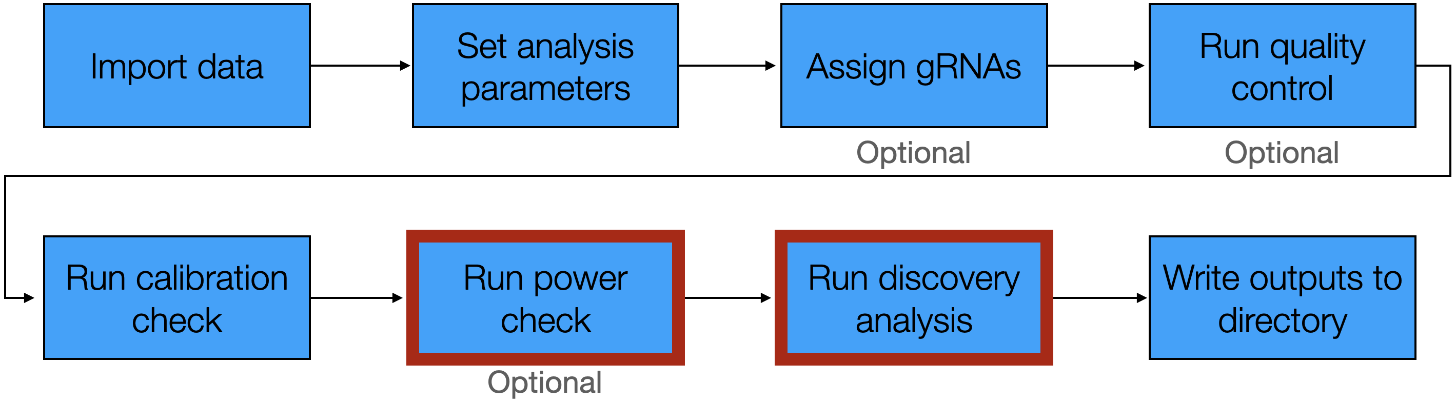
6 Run power check and discovery analysis
The next steps of the pipeline are to run the power check and the discovery analysis. The power check entails applying sceptre to analyze positive control pairs — pairs for which we know there is an association between the target and the response — to ensure that sceptre is capable of detecting true associations. The discovery analysis, meanwhile, involves applying sceptre to analyze discovery pairs, or target-response pairs whose association status we do not know but seek to learn. Identifying associations among the discovery pairs is the primary objective of the single-cell CRISPR screen analysis. We explicate both the power check and discovery analysis in this chapter given the similarity of these two analyses.
We load the sceptre, sceptredata, dplyr, and cowplot packages.
We initialize sceptre_objects corresponding to the high-MOI CRISPRi data and low-MOI CRISPRko data. We call all pipeline functions that precede run_power_check() and run_discovery_analysis() (namely, import_data(), set_analysis_parameters(), assign_grnas(), run_qc(), and run_calibration_check()) on both datasets.
# low-MOI CRISPRko data
# 1. import data
data(lowmoi_example_data)
sceptre_object_lowmoi <- import_data(
  response_matrix = lowmoi_example_data$response_matrix,
  grna_matrix = lowmoi_example_data$grna_matrix,
  extra_covariates = lowmoi_example_data$extra_covariates,
  grna_target_data_frame = lowmoi_example_data$grna_target_data_frame,
  moi = "low"
)
positive_control_pairs_lowmoi <- construct_positive_control_pairs(
  sceptre_object = sceptre_object_lowmoi
)
discovery_pairs_lowmoi <- construct_trans_pairs(
  sceptre_object = sceptre_object_lowmoi,
  positive_control_pairs = positive_control_pairs_lowmoi,
  pairs_to_exclude = "pc_pairs"
)

# 2-5. set analysis parameters, assign gRNAs, run qc, run calibration check
sceptre_object_lowmoi <- sceptre_object_lowmoi |>
  set_analysis_parameters(
    discovery_pairs = discovery_pairs_lowmoi,
    positive_control_pairs = positive_control_pairs_lowmoi
  ) |>
  assign_grnas() |>
  run_qc(p_mito_threshold = 0.075) |>
  run_calibration_check(parallel = TRUE)
# high-MOI CRISPRi data
# 1. import data
data(highmoi_example_data); data(grna_target_data_frame_highmoi)
sceptre_object_highmoi <- import_data(
response_matrix = highmoi_example_data$response_matrix,
grna_matrix = highmoi_example_data$grna_matrix,
grna_target_data_frame = grna_target_data_frame_highmoi,
moi = "high",
extra_covariates = highmoi_example_data$extra_covariates,
response_names = highmoi_example_data$gene_names
)
positive_control_pairs_highmoi <- construct_positive_control_pairs(
sceptre_object = sceptre_object_highmoi)
discovery_pairs_highmoi <- construct_cis_pairs(sceptre_object_highmoi,
positive_control_pairs = positive_control_pairs_highmoi,
distance_threshold = 5e6
)
# 2-4. set analysis parameters, assign gRNAs, run qc, run calibration check
sceptre_object_highmoi <- sceptre_object_highmoi |>
set_analysis_parameters(
discovery_pairs = discovery_pairs_highmoi,
positive_control_pairs = positive_control_pairs_highmoi,
side = "left"
) |>
assign_grnas(parallel = TRUE) |>
run_qc(p_mito_threshold = 0.075) |>
run_calibration_check(parallel = TRUE)We are now ready to run the power check and discovery analysis.
6.1 Run power check
We run the power check by calling the function run_power_check(), which takes the arguments sceptre_object (required), output_amount (optional), print_progress (optional), and parallel (optional). output_amount controls the amount of information that run_power_check() returns; see Section 5.5 of Run calibration check for more information about this argument. print_progress and parallel are logical values indicating whether to print progress updates and run the computation in parallel, respectively. We run the power check on the low-MOI CRISPRko data.
sceptre_object_lowmoi <- run_power_check(
  sceptre_object = sceptre_object_lowmoi,
  parallel = TRUE
)
We call plot() on the resulting sceptre_object to visualize the outcome of the power check.
plot(sceptre_object_lowmoi)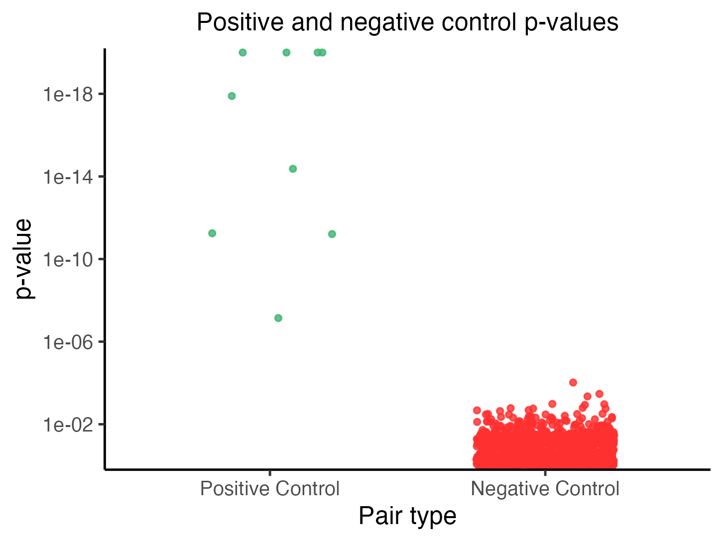
We described how to interpret this plot in Section 6 of The whole game. Briefly, each point represents a pair, and the vertical position of a given point indicates the p-value of the corresponding pair. Points in the left (resp., right) column are positive control (resp, negative control) pairs. The positive control p-values should be generally smaller (i.e., more significant) than the negative control p-values.
6.2 Run discovery analysis
We run the discovery analysis by calling the function run_discovery_analysis(), which takes the same arguments as run_power_check(). We illustrate this function on the low-MOI CRISPRko data.
sceptre_object_lowmoi <- run_discovery_analysis(
  sceptre_object = sceptre_object_lowmoi,
  parallel = TRUE
)
We can visualize the outcome of the discovery analysis by calling plot() on the resulting sceptre_object.
plot(sceptre_object_lowmoi)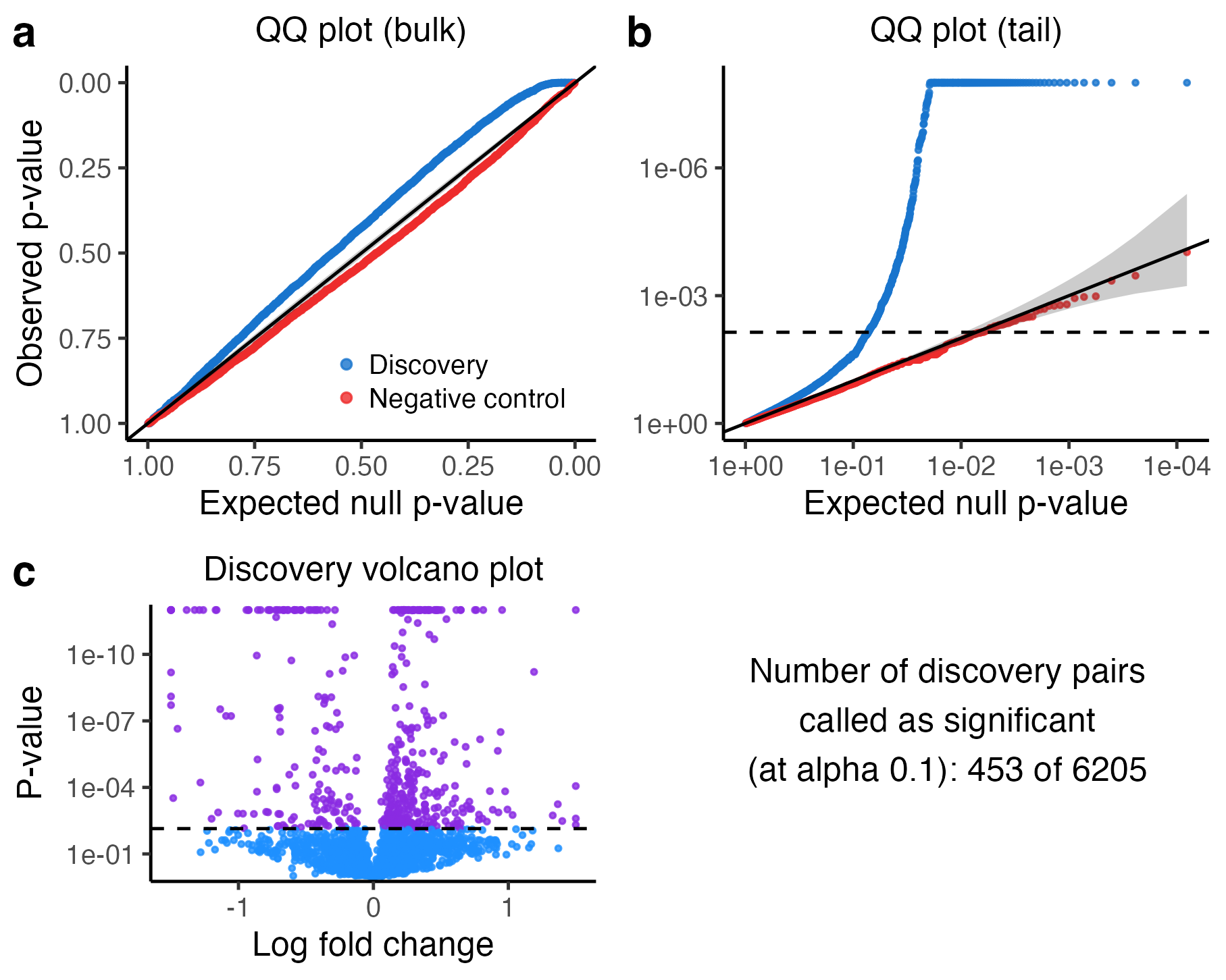
We described how to interpret this plot in Section 7 of The whole game. Briefly, the top left (resp. right) panel is a QQ plot of the negative control p-values and the discovery p-values plotted on an untransformed (resp., transformed) scale. The bottom left panel plots the p-value of each discovery pair against its log-2-fold-change. Finally, the bottom right panel displays the number of discoveries that sceptre makes on the discovery set (after applying the multiplicity correction).
6.3 Visualizing the results for individual pairs
We can visualize the results for an individual target-response pair by calling the function plot_response_grna_target_pair(). plot_response_grna_target_pair() takes as input a sceptre_object, a response ID response_id, and a gRNA target grna_target. plot_response_grna_target_pair() creates two side-by-side violin plots depicting the expression level of the response. The left (resp., right) violin plot shows the expression level of the response in treatment (resp., control) cells. (When control_group is set to "nt_cells", the control cells are those containing an NT gRNA, whereas when control_group is set to "complement", the control cells are those that do not contain a gRNA targeting the given site.) The response expression vector is normalized by dividing by the library size (i.e., response_n_umis), adding a pseudo-count of 1, and then taking a log transformation. Finally, if the given pair has been analyzed (either as part of the power check or the discovery analysis), a p-value for the test of association between the target and response is displayed.
To illustrate use of this function, we create the above-described plot for two pairs: the positive control pair consisting of gRNA target “CMTM6” and response “CMTM6”, and the discovery pair consisting of gRNA target “STAT3” and response “ACADVL.” We use plot_grid() from cowplot to render the plots side-by-side.
pc_pair <- plot_response_grna_target_pair(sceptre_object = sceptre_object_lowmoi,
                                          response_id = "CMTM6",
                                          grna_target = "CMTM6")
disc_pair <- plot_response_grna_target_pair(sceptre_object = sceptre_object_lowmoi,
                                            response_id = "ACADVL",
                                            grna_target = "STAT3")
plot_grid(pc_pair, disc_pair)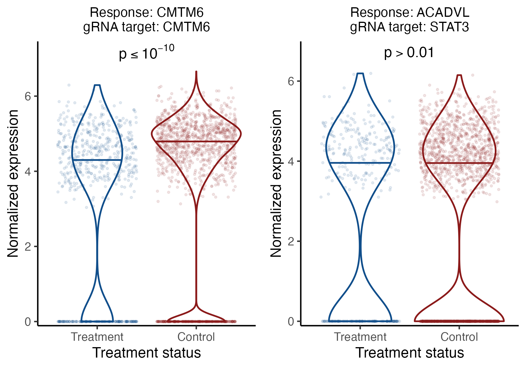
Finally, if grna_integration_strategy has been set to "singleton", then an individual gRNA ID should be passed to grna_target in lieu of of a gRNA target.
6.4 Inspecting the results
We can obtain a data frame containing the results by calling get_result() on the sceptre_object, setting the parameter analysis to the name of the function whose results we are querying. For example, we can obtain the discovery results as follows.
discovery_result <- get_result(
  sceptre_object = sceptre_object_lowmoi,
  analysis = "run_discovery_analysis"
)
head(discovery_result)
response_id grna_target n_nonzero_trt n_nonzero_cntrl pass_qc p_value
<char> <char> <int> <int> <lgcl> <num>
1: JAK2 STAT1 112 1557 TRUE 1.000000e-250
2: PSMB9 IFNGR1 873 1801 TRUE 3.381202e-155
3: PSMB9 JAK2 706 1801 TRUE 4.456437e-145
4: STAT1 IFNGR2 821 1819 TRUE 1.918728e-127
5: STAT1 IFNGR1 898 1819 TRUE 7.934591e-127
6: STAT1 JAK2 714 1819 TRUE 1.342549e-122
log_2_fold_change significant
<num> <lgcl>
1: -1.3840723 TRUE
2: -0.8561766 TRUE
3: -0.9410000 TRUE
4: -0.6669393 TRUE
5: -0.6371647 TRUE
6: -0.7134929 TRUEThe data frame discovery_result contains the columns response_id, grna_target, n_nonzero_trt, n_nonzero_cntrl, pass_qc, p_value, log_2_fold_change, and significant; see Section 5.2 of Run calibration check for a description of these columns. The rows are ordered according to p_value. Pairs called as significant are stored in the top rows of the data frame; pairs called as insignificant are stored in the middle rows; and pairs filtered out by pairwise QC are stored in the bottom rows. (The latter pairs have a value of NA in the p_value, log_2_fold_change, and significant columns.)
The format of the result data frame is slightly different when we use the “singleton” gRNA integration strategy rather than the default “union” strategy. To illustrate, we again analyze the low-MOI CRISPRko data, this time setting grna_integration_strategy to "singleton" in set_analysis_parameters(). We then call assign_grnas(), run_qc(), and run_discovery_analysis().
sceptre_object_lowmoi_singleton <- sceptre_object_lowmoi |>
  set_analysis_parameters(
    discovery_pairs = discovery_pairs_lowmoi,
    positive_control_pairs = positive_control_pairs_lowmoi,
    grna_integration_strategy = "singleton"
  ) |>
  assign_grnas() |>
  run_qc(p_mito_threshold = 0.075) |>
  run_discovery_analysis(parallel = TRUE)
The result data frame obtained via get_result() contains the additional column grna_id. Each row of this data frame corresponds to an individual gRNA-response pair (as opposed to target-response pair).
discovery_result <- get_result(
  sceptre_object = sceptre_object_lowmoi_singleton,
  analysis = "run_discovery_analysis"
)
head(discovery_result)
response_id grna_id grna_target n_nonzero_trt n_nonzero_cntrl pass_qc
<char> <char> <char> <int> <int> <lgcl>
1: JAK2 IFNGR1g3 IFNGR1 141 1557 TRUE
2: JAK2 IRF1g4 IRF1 94 1557 TRUE
3: PSMB9 IFNGR1g3 IFNGR1 304 1801 TRUE
4: STAT1 IFNGR2g2 IFNGR2 280 1819 TRUE
5: UBE2L6 IFNGR2g1 IFNGR2 375 1794 TRUE
6: PSMB9 IFNGR2g1 IFNGR2 384 1801 TRUE
p_value log_2_fold_change significant
<num> <num> <lgcl>
1: 1.000000e-250 -1.5869800 TRUE
2: 1.000000e-250 -1.7962142 TRUE
3: 1.000000e-250 -1.2386121 TRUE
4: 1.000000e-250 -0.7611831 TRUE
5: 1.000000e-250 -0.8712660 TRUE
6: 9.742212e-106 -1.2076649 TRUEWe can filter for a given target to view the p-values of the individual gRNAs targeting that target. For example, we filter the result data frame for rows containing response ID “PSMB9” and gRNA target “IFNGR2,” displaying the columns response_id, grna_id, grna_target, p_value, significant, and n_nonzero_trt.
discovery_result |>
  filter(response_id == "PSMB9", grna_target == "IFNGR2") |>
  select(response_id, grna_id, grna_target, p_value, significant, n_nonzero_trt)
response_id grna_id grna_target p_value significant n_nonzero_trt
<char> <char> <char> <num> <lgcl> <int>
1: PSMB9 IFNGR2g1 IFNGR2 9.742212e-106 TRUE 384
2: PSMB9 IFNGR2g2 IFNGR2 9.280088e-50 TRUE 286
3: PSMB9 IFNGR2g3 IFNGR2 1.424416e-17 TRUE 115
4: PSMB9 IFNGR2g4 IFNGR2 3.200000e-02 FALSE 12The individual gRNAs that target “IFNGR2” are “IFNGR2g1,” “IFNGR2g2,” IFNGR2g3,” and “IFNGR2g4.” All produce a significant association except “IFNGR2g4.” The latter likely does not produce a significant association because the pair consisting of gRNA IFNGR2g4 and response PSMB9 has a smaller effective sample size than the other pairs (as quantified by n_nonzero_trt).
We additionally can call print() on the updated sceptre_object to print information about the status of the analysis to the console.
print(sceptre_object_lowmoi)An object of class sceptre_object.
Attributes of the data:
• 20729 cells (15348 after cellwise QC)
• 299 responses
• Low multiplicity-of-infection
• 101 targeting gRNAs (distributed across 26 targets)
• 9 non-targeting gRNAs
• 6 covariates (bio_rep, grna_n_nonzero, grna_n_umis, response_n_nonzero, response_n_umis, response_p_mito)
Analysis status:
✓ import_data()
✓ set_analysis_parameters()
✓ assign_grnas()
✓ run_qc()
✓ run_calibration_check()
✓ run_power_check()
✓ run_discovery_analysis()
Analysis parameters:
• Discovery pairs: data frame with 7765 pairs (6205 after pairwise QC)
• Positive control pairs: data frame with 9 pairs (9 after pairwise QC)
• Sidedness of test: both
• Control group: non-targeting cells
• Resampling mechanism: permutations
• gRNA integration strategy: union
• Resampling approximation: skew normal
• Multiple testing adjustment: BH at level 0.1
• N nonzero treatment cells threshold: 7
• N nonzero control cells threshold: 7
• Formula object: log(response_n_nonzero) + log(response_n_umis) + bio_rep
gRNA-to-cell assignment information:
• Assignment method: maximum
• Mean N cells per gRNA: 188.45
• Mean N gRNAs per cell (MOI): not computed when using "maximum" assignment method
Summary of results:
• N negative control pairs called as significant: 0/6205
• Mean log-2 FC for negative control pairs: -0.0027
• Median positive control p-value: 1.3e-18
• N discovery pairs called as significant: 453/6205The third and fourth entries under the field “Summary of results” provide information about the power check and discovery analysis, respectively.
6.5 Writing the outputs to a directory
We can write all outputs (i.e., results and plots) of an analysis to a directory on disk via the function write_outputs_to_directory(). See Section 8 of The whole game for a description of this function.